

By Urban Demographics | Rafael H. M. Pereira Researcher (Ipea)
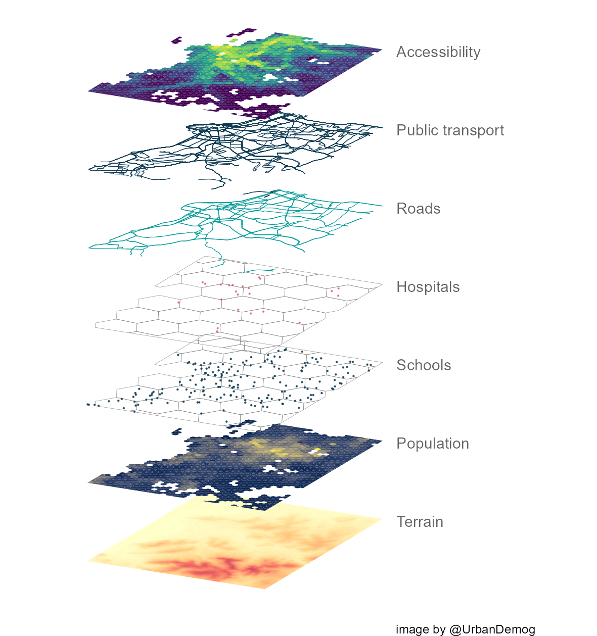
I like figures of map layers to illustrate the many different types of data sets we combine to do urban and transport modeling. And oftentimes I get obsessed with like making maps that are reproducible with code in R. In this post I’ll be sharing a reproducible example showing how to create a figure of stacked maps like this one below.
Quick background: In 2014, I was trying to find a way to create map layers in R. This was before the sf library was created. Most of us were using the sp library for handling spatial data and Barry Rowlingson was super helpful, as usual. I used Barry’s suggestion to create a reproducible example so I could use it latter, but then sf was created and it completely changed how we do spatial analysis in R. Since then, Lauren O’brien proposed a simple way to tilt and stack sf objects and Stefan Jünger created an elegant function to do this. I’ll be using Stefan’s function in my example below.
ad libraries
library(easypackages)
easypackages::packages("sf",
                       "raster",
                       "stars",
                       "r5r",
                       "geobr",
                       "aopdata",
                       "gtfs2gps",
                       "ggplot2",
                       "osmdata",
                       "h3jsr",
                       "viridisLite",
                       "ggnewscale",
                       "dplyr",
                       "magrittr",
                       prompt = FALSE
                       )
Functions to tilt sf
Original function created by Stefan Jünger.
rotate_data <- function(data, x_add = 0, y_add = 0) {

  shear_matrix <- function(){ matrix(c(2, 1.2, 0, 1), 2, 2) }

  rotate_matrix <- function(x){
    matrix(c(cos(x), sin(x), -sin(x), cos(x)), 2, 2)
  }
  data %>%
    dplyr::mutate(
      geometry = .$geometry * shear_matrix() * rotate_matrix(pi/20) + c(x_add, y_add)
    )
}

rotate_data_geom <- function(data, x_add = 0, y_add = 0) {
  shear_matrix <- function(){ matrix(c(2, 1.2, 0, 1), 2, 2) }

  rotate_matrix <- function(x) {
    matrix(c(cos(x), sin(x), -sin(x), cos(x)), 2, 2)
  }
  data %>%
    dplyr::mutate(
      geom = .$geom * shear_matrix() * rotate_matrix(pi/20) + c(x_add, y_add)
    )
}
Load data
We’ll be using a few data sets available from the packages used here. The first thing we need to do is to load the data and crop them to make sure they have the same extent.
### get terrain data ----------------

  # read terrain raster and calculate hill Shade
  dem <- stars::read_stars(system.file("extdata/poa/poa_elevation.tif", package = "r5r"))
  dem <- st_as_sf(dem)

  # crop
  bbox <- st_bbox(dem)


### get public transport network data ----------------

  gtfs <- gtfs2gps::read_gtfs( system.file("extdata/poa/poa.zip", package = "r5r") )
  gtfs <- gtfs2gps::gtfs_shapes_as_sf(gtfs)

  # crop
  gtfs <- gtfs[bbox,]
  gtfs <- st_crop(gtfs, bbox)
  plot(gtfs['shape_id'])


### get OSM data ----------------

  # roads from OSM
  roads <- opq('porto alegre') %>%
           add_osm_feature(key = 'highway',
                           value = c("motorway", "primary","secondary")) %>% osmdata_sf()

  roads <- roads$osm_lines

  # crop
  roads2 <- roads[bbox,]
  roads2 <- st_crop(roads2, bbox)
  plot(roads2['osm_id'])


### get H3 hexagonal grid ----------------

  # get poa muni and hex ids
  poa <- read_municipality(code_muni = 4314902 )
  hex_ids <- h3jsr::polyfill(poa, res = 7, simple = TRUE)

  # pass h3 ids to return the hexagonal grid
  hex_grid <- h3jsr::h3_to_polygon(hex_ids, simple = FALSE)
  plot(hex_grid)

  # crop
  hex_grid <- hex_grid[bbox,]
  hex <- st_crop(hex_grid, bbox)
  plot(hex)


### get land use data from AOP project ----------------
#' more info at https://www.ipea.gov.br/acessooportunidades/en/

  landuse <- aopdata::read_access(city = 'poa', geometry = T, mode='public_transport')

  # crop
  landuse <- landuse[bbox,]
  landuse <- st_crop(landuse, bbox)
  plot(landuse['CMATT30'])

  # hospitals
  # generate one point per hospital in corresponding hex cells
  df_temp <- subset(landuse, S004>0)
  hospitals <- st_sample(x = df_temp, df_temp$S004, by_polygon = T)
  hospitals <- st_sf(hospitals)
  hospitals$geometry <- st_geometry(hospitals)
  hospitals$hospitals <- NULL
  hospitals <- st_sf(hospitals)
  plot(hospitals)

  # schools
  # generate one point per schools in corresponding hex cells
  df_temp <- subset(landuse, E001>0)
  schools <- st_sample(x = df_temp, df_temp$E001, by_polygon = T)
  schools <- st_sf(schools)
  schools$geometry <- st_geometry(schools)
  schools$schools <- NULL
  schools <- st_sf(schools)
  plot(schools)
Plot
### plot  ----------------

# annotate parameters
x = -141.25
color = 'gray40'

temp1 <- ggplot() +

        # terrain
        geom_sf(data = dem %>% rotate_data(), aes(fill=poa_elevation.tif), color=NA, show.legend = FALSE) +
        scale_fill_distiller(palette = "YlOrRd", direction = 1) +
        annotate("text", label='Terrain', x=x, y= -8.0, hjust = 0, color=color) +
        labs(caption = "image by @UrbanDemog")

temp2 <- temp1 +

        # pop income
        new_scale_fill() +
        new_scale_color() +
        geom_sf(data = subset(landuse,P001>0) %>% rotate_data(y_add = .1), aes(fill=R001), color=NA, show.legend = FALSE) +
        scale_fill_viridis_c(option = 'E') +
        annotate("text", label='Population', x=x, y= -7.9, hjust = 0, color=color) +

        # schools
        geom_sf(data = hex %>% rotate_data(y_add = .2), color='gray50', fill=NA, size=.1) +
        geom_sf(data = schools %>% rotate_data(y_add = .2), color='#0f3c53', size=.1, alpha=.8) +
        annotate("text", label='Schools', x=x, y= -7.8, hjust = 0, color=color) +

        # hospitals
        geom_sf(data = hex %>% rotate_data(y_add = .3), color='gray50', fill=NA, size=.1) +
        geom_sf(data = hospitals %>% rotate_data(y_add = .3), color='#d5303e', size=.1, alpha=.5) +
        annotate("text", label='Hospitals', x=x, y= -7.7, hjust = 0, color=color) +

        # OSM
        geom_sf(data = roads2 %>% rotate_data(y_add = .4), color='#019a98', size=.2) +
        annotate("text", label='Roads', x=x, y= -7.6, hjust = 0, color=color) +

        # public transport
        geom_sf(data = gtfs %>% rotate_data(y_add = .5), color='#0f3c53', size=.2) +
        annotate("text", label='Public transport', x=x, y= -7.5, hjust = 0, color=color) +

        # accessibility
        new_scale_fill() +
        new_scale_color() +
        geom_sf(data = subset(landuse, P001>0) %>% rotate_data(y_add = .6), aes(fill=CMATT30), color=NA, show.legend = FALSE) +
        scale_fill_viridis_c(direction = 1, option = 'viridis' ) +
        theme(legend.position = "none") +
        annotate("text", label='Accessibility', x=x, y= -7.4, hjust = 0, color=color) +
        theme_void() +
        scale_x_continuous(limits = c(-141.65, -141.1))


# save plot
ggsave(plot = temp2, filename = 'map_layers.png',
       dpi=200, width = 15, height = 16, units='cm')